Computing the integrated solid angle of a particle

This tutorial show how to crete a configuration and computing the integrated solid angle subtended by a particle’s trajectory along phi with certain discretization, and plotting it.

\(\int_\Phi \Omega R d \Phi\)

Useful for reconstructing emissivity.

We start by loading ITER’s configuration (built-in in tofu)

import matplotlib.pyplot as plt
import numpy as np
import tofu as tf


config = tf.load_config("ITER")

We define the particles properties and trajectory. Let’s suppose we have the data for three points of the trajectory, the particle moves along X from point (5, 0, 0) in cartesian coordinates, to (6, 0, 0) and finally to (7, 0, 0). At the end point the particle radius seems to be a bit bigger (\(2 \mu m\) instead of \(1 \mu m\))

part_rad = np.r_[.0001, .0001, .0002]*2

part_traj = np.array([[5.0, 0.0, 0.0],
                      [6.0, 0.0, 0.0],
                      [7.0, 0.0, 0.0]], order="F").T

Let’s set some parameters for the discretization for computing the integral: resolutions in (R, Z, Phi) directions and the values to only compute the integral on the core of the plasma.

r_step = z_step = phi_step = 0.02  # 1 cm resolution along all directions
Rminmax = np.r_[4.0, 8.0]
Zminmax = np.r_[-5., 5.0]

Let’s compute the integrated solid angle: the function returns the points in (R,Z) of the discretization, the integrated solid angle on those points, the indices to reconstruct the discretization in all domain and a the volume unit \(dR * dZ\).

pts, sa_map, ind, vol = tf.geom._GG.compute_solid_angle_map(part_traj,
                                                            part_rad,
                                                            r_step,
                                                            z_step,
                                                            phi_step,
                                                            Rminmax,
                                                            Zminmax)

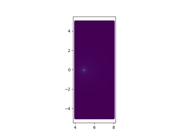
Now we can plot the results the first point on the trajectory

fig1, ax = plt.subplots()

ax.scatter(pts[0, :], pts[1, :],    # R and Z coordinates
           marker="s",              # each point is a squared pixel
           edgecolors=None,         # no boundary for smooth plot
           s=10,                    # size of pixel
           c=sa_map[:, 0].flatten(),  # pixel color is value of int solid angle
           )
ax.set_aspect("equal")
plt.show()

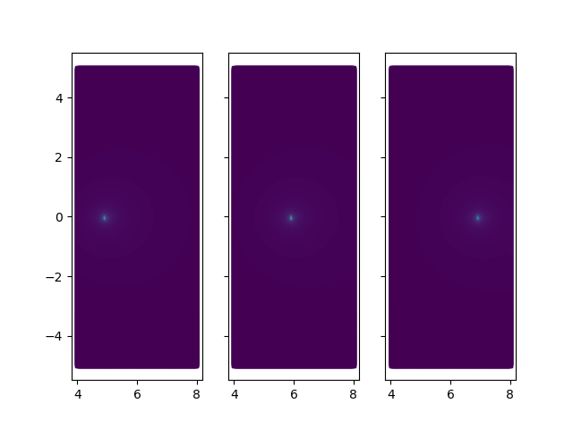
or the three points in the trajectory

fig2, list_axes = plt.subplots(ncols=3, sharey=True)

# Now we can plot the results for all points on the trajectory
for (ind, ax) in enumerate(list_axes):
    ax.scatter(pts[0, :], pts[1, :],
               marker="s",
               edgecolors=None,
               s=10,
               c=sa_map[:, ind].flatten(),  # we change particle number
               )
    ax.set_aspect("equal")


plt.show()

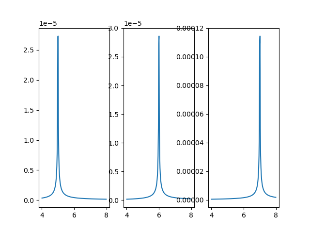
Now let’s see the 1D profile of all particles for z = 0.

izero = np.abs(pts[1, :]) < z_step

fig3, list_axes = plt.subplots(ncols=3, sharey=False)

for (ind, ax) in enumerate(list_axes):
    ax.plot(pts[0, izero], sa_map[izero, ind])

plt.show()